Benchmarking Regression algorithms with Apache Spark
On this page we give an overview of how we conducted benchmarks on Linear Regression in Spark, on generated, synthetic, normally distributed data of a range of sizes under different settings on the Cray-Urika GX. Broadly speaking, our benchmarks were conducted for two types of data sizes, ‘Large n, small p’, where n, the number of rows, is much larger than the number of columns p, as well as the opposite case of Large p, small n. These two scenarios are the most commonly encountered in practical applications. ‘Large n, small p’ is typically encountered when a small amount of data is collected frequently over a large number of instances, for example transactional data. ‘Large p and small n’, or high dimensional datasets arise in applications such as genomic data.
We run the benchmarks via a bash script which calls a python file under different input parameters through argparse. The Python file contains the PySpark script that runs the actual linear regression algorithm to be benchmarked. The variable settings are:
‘coresmax’, number of maximum cores. Cray-Urika GX has 324 cores in total. You can set this number to be greater than 324, but it’s just effectively capped at 324.
‘executorcores’, number of cores used by each executor or node. Spark has 36 CPU cores per node. Note this must be less than ‘coresmax’ otherwise Spark will not have enough cores to initiate and return an error.
‘executormemory’, amount of memory assigned to each executor. In general (min(coresmax, 324)/executorcores’)*executormemory<=1800 should be true if you want Spark to run on coresmax cores, otherwise Spark will scale down on the number of cores used due to the lack of memory. In general for other clusters, replace 324 by the (maximum) number of CPU cores and 1800 by the total memory of your cluster, respectively.
‘n’, number of rows in the data
‘p’, number of columns in the data
‘maxiter’, maximum number of iterations of the linear regression
‘lamda’, parameter controlling how much penalisation you want
‘alpha’, parameter between 0 and 1 controlling type of parametrisation (elastic net). 1 denotes LASSO/L1 penalisation, 0 denotes Ridge/L2 penalisation. Any number between 0 and 1 is a weighted linear combination of both.
The bash code looks like this:
for i in {4..9}; do for j in {1..2}; do for k in 1 5 10 22; do for l in 1 10 100; do for z in 0 0.1; do for x in 0 0.5 1; do for c in 1 4 16 36; do for v in 1 16 256 512 36000; do
    if [ $v -ge $c ]; then
    spark-submit LRLargeNsmallPBenchmark.py --n $((10**$i)) --p $((10**$j)) --executormemory $((10*$k))g --maxiter $((10*$l)) --lamda $z --alpha $x --executorcores $c --coresmax $v;
    else
    	echo coresmax $v smaller than executorcores $c
    fi
done;
done;
done;
done;
done;
done;
done;
done
We have 4 versions of (Linear Regression, Logistic Regression, Large n small p, Large p small n) of the Python file, but common to all of them, we start by importing modules, defining the Spark context and setting up argparse so the input parameters can be passed in correctly.
import numpy as np
import findspark
findspark.init()
import scipy as scipy
from pyspark.sql import SparkSession
from pyspark.sql import Row
from pyspark.sql.types import *
from pyspark.sql.functions import *
from pyspark.ml.linalg import DenseVector
from pyspark.ml.feature import StandardScaler
from pyspark.ml.regression import LinearRegression
from pyspark.mllib.regression import LinearRegressionWithSGD
from pyspark.mllib.regression import LabeledPoint
from pyspark.mllib.feature import StandardScaler
from pyspark import SparkConf, SparkContext

import argparse
parser = argparse.ArgumentParser()
parser.add_argument('--coresmax', nargs='?', const=36000, type=int, default=36000)
parser.add_argument('--executorcores', nargs='?', const=36, type=int, default=36)
parser.add_argument('--drivermemory', nargs='?', const='96g', type=str, default='96g')
parser.add_argument('--executormemory', nargs='?', const='96g', type=str, default='96g')
parser.add_argument('--n', nargs='?', const=10000000000, type=int, default=10000000000)
parser.add_argument('--p', nargs='?', const=100, type=int, default=100)
parser.add_argument('--maxiter', nargs='?', const=100, type=int, default=100)
parser.add_argument('--lamda', nargs='?', const=0, type=float, default=0)
parser.add_argument('--alpha', nargs='?', const=0, type=float, default=0)
args = parser.parse_args()
print(args)

spark = SparkSession.builder    .master("mesos://zk://zoo1:2181,zoo2:2181,zoo3:2181/mesos")    .appName("Linear Regression Model SGD")    .config("spark.cores.max", args.coresmax)    .config("spark.executor.cores", args.executorcores)    .config("spark.driver.memory.", args.drivermemory)    .config("spark.executor.memory", args.executormemory)    .getOrCreate()

sc = spark.sparkContext


print(sc._conf.getAll()) #print settings to double check

import time
time.sleep(10)
print('wait over')
Again if running Mesos we want to let Python wait for 10 seconds before running code on data because Mesos takes a few seconds to initialise.
Large n, small p
The basic idea is to initialise a dataframe with just the row label, and then generate columns of the desired dataframe iteratively via the select method in Spark, until we reach the number of columns we want.
from pyspark.sql.functions import rand, randn


n=args.n
p=args.p
meanmag=10
stdmag=7
coefmag=5
noisestd=3

dfgen = spark.range(0, n) #initialise dataframe

coefs=coefmag*np.random.uniform(low=-1, high=1, size=p) #generate coefficients
interceptcoef=coefmag*np.random.uniform(low=-1, high=1) #generate intercept coefficient

print(coefs)
print(interceptcoef)


#generate p columns of feature data
for i in range(p):
    np.random.seed(i)
    stdmagrand=stdmag*np.random.rand() #standard deviation of ith column, generated via N(0, stdmag)
    meanmagrand=meanmag*np.random.randn() #mean of ith column, generated via N(0, meanmag)
    #print(stdmagrand)
    #print(meanmagrand)
    #select everything already in the dataframe, plus the new generated column 'X_i'
    dfgen=dfgen.select('*', (meanmagrand+stdmagrand*randn(seed=i)).alias("X"+str(i)))

dfgen=dfgen.drop("id")

dfgen.take(1)

#next we need to add the response column, can't do matrix multiplication with a dataframe so need iterative approach
#first iteration we add the intercept, noise and the first feature column's contribution to the response
dfgen=dfgen.select((interceptcoef+coefs[0]*dfgen["X0"]+noisestd*randn(seed=2*p+4)).alias("Y"+str(0)), '*')

#subsequently add contributions from the other columns sequentially and iteractively to the response
for i in range(p-1):
    dfgen=dfgen.select((dfgen["Y"+str(i)]+coefs[i+1]*dfgen["X"+str(i+1)]).alias("Y"+str(i+1)), '*')
    #drop the previous value of the response at each iteration
    dfgen=dfgen.drop("Y"+str(i))

print(dfgen.take(1))

print('done')
For each column, we generate n independent samples from a normal distribution with mean ‘meanmagrand’ and standard deviation ‘stdmagrand’, which in turn are generated from N(0, meanmag) and N(0, stdmag) respectively. ‘meanmag’ and ‘stdmag’ are defined by the user and basically gives you some control of how large you want the columns to be while still keeping the columns generated from different distributions and the data random. Columns are appended to the initial dataframe via ‘select’. The columns are named ‘X0’, ‘X1’, ‘X2’, …
It’s not simple to do matrix multiplication or dot product in a Spark dataframe, so the response variable is generated as follows: first we require coefficient values of the model we want to fit, which are generated via an uniform distribution U(-coefmag, coefmag) where again coefmag is a parameter defined by the user which controls how large the intercept is. Next, once we generate the data, we initialise another column called ‘Y0’ which is the intercept+coefs[0]X0+noise, and iteratively add the contribution from the other columns e.g. Y5=Y4+coefs[5]X5 until we reach the last column.
The actual model fitting part is relatively straightforward. We time how long it takes for Spark to fit the linear regression and write ‘results’ which includes the benchmark time as well as parameters used in this run to a csv file.
import time
import datetime

start = time.time()
print(datetime.datetime.now())
# Initialize `lr`
print('Im running')
lrgen = LinearRegression(labelCol="label", featuresCol="features", maxIter=args.maxiter, regParam=args.lamda, elasticNetParam=args.alpha)
# Fit the data to the model
linearModelgen = lrgen.fit(dfgenY)
end = time.time()
print(datetime.datetime.now())
timetaken=end-start
print(timetaken)
print(linearModelgen.coefficients)
print(linearModelgen.intercept)
print(linearModelgen.summary.rootMeanSquaredError)
print('done')

results=[args.coresmax, args.executorcores, args.drivermemory, args.executormemory, args.n, args.p, args.maxiter, timetaken, linearModelgen.summary.rootMeanSquaredError, input_data_gen.getNumPartitions(), args.lamda, args.alpha]

import csv
with open("MLLRresultsbonus.txt", "a") as f:
    wr = csv.writer(f)
    wr.writerow(results)
f.close()
Large p, small n
The code used for the large p, small n case differs significantly from the large n, small p case in the data generating process, but is similar in the other parts. Iteratively adding columns to a dataframe becomes quite slow when p gets to over about 1000 so it’s not feasible to use the same method to generate a large p, small n dataset. So instead of iteratively adding columns we iteratively append rows to the dataset instead. To do this we generate a row in numpy first, turn it into an rdd via SparkContext.parallelize and append it to the existing dataset via SparkContext.union. An obvious weakness in this approach is that numpy isn’t parallelised by Spark but Spark does not offer easy ways to append rows to a dataset due to the rdd data structure.
from pyspark.sql.functions import rand, randn
from pyspark.sql import Row


n=args.n
p=args.p #10m seems to be about the limit

print([n,p])

meanmag=10
mean=meanmag*np.random.randn(p) #generate means of feature columns
print('is numpy slow') #dont simulate from np.multivariate.normal, it's very slow. Instead simulate from randn and add the mean and np.multiply for diagonal covariance
std=7
stdvec=np.random.uniform(low=0.1, high=std, size=p) #generate std of feature columns
coefmag=5 #maximum 'magnitude' of coefficients
noisestd=3 #standard deviance of noise

coef=coefmag*np.random.uniform(low=-1, high=1, size=p) #generate coefficients
interceptcoef=coefmag*np.random.uniform(low=-1, high=1, size=1) #generate intercept coefficient

print('print coefficients')
#print(coef)
#print(interceptcoef)

features=mean+np.multiply(np.random.randn(p), stdvec)
#generate p independent N(0,1) samples, multiply componentwise with the vector of standard deviance, and add the vector of means

#print(features)

response=interceptcoef+np.dot(coef, features)+noisestd*np.random.randn()
#print(response)
#print(features)

row0=np.concatenate([response, features])


rdd0 = sc.parallelize([row0.tolist()]) #the square brackets somehow convinces spark to initialise this array as a row rather than column
#print(rdd0.collect())

print('start')

for i in range(n-1):
    features=mean+np.multiply(np.random.randn(p), stdvec)
    #print(features[0])
    response=interceptcoef+np.dot(coef, features)+noisestd*np.random.randn()
    #print(response)
    row=np.concatenate([response, features])
    #print(row)
    #print(row.reshape(1, row.shape[0]))
    rdd = sc.parallelize([row.tolist()])
    #print(rdd.collect())
    rdd0=sc.union([rdd0,rdd])
    #row0=row

#print('entire data')
#print(rdd0.collect())


# Define the `input_data`
input_data_gen = rdd0.map(lambda x: (x[0], DenseVector(x[1:])))
#input_data_gen = rdd0.map(lambda x: x[1])


#print(input_data_gen.collect())


# Replace `df` with the new DataFrame
dfgenY = spark.createDataFrame(input_data_gen, ["label", "features"])
Notable results
Runtime vs data size
| n | p | Runtime(s) |
|---|---|---|
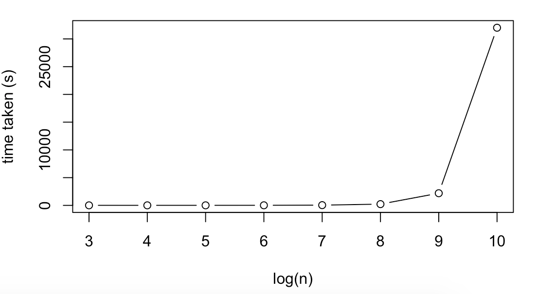
| 10^3 | 100 | 9.48 |
| 10^4 | 100 | 9.06 |
| 10^5 | 100 | 10.22 |
| 10^6 | 100 | 17.08 |
| 10^7 | 100 | 43.01 |
| 10^8 | 100 | 226.57 |
| 10^9 | 100 | 2191.76 |
| 10^10 | 100 | 32018.55 |
| 100 | 10^5 | 2534.42 |
| 100 | 10^6 | 5176.72 |
We present some notable benchmarks for linear regression. Here the total number of cores was kept at the 324 maximum for each run. For small n the bottleneck does not appear to be related to the size of the data, as from n=10^3 to 10^5 the Runtime was relatively constant. Overall Spark seems to run on large n, small p datasets more efficiently in terms of how much computational time scales with runtime. This is likely because large p, small n datasets require penalisation (feature selection) over a much larger number of columns which slows the algorithm down.
Runtime vs number of cores used
The inverse of runtime time seems to vary linearly as the number of cores increase, at least provided there’s enough memory. The data used here was n=10^8, p=10, with 100gb memory per executor, and the algorithm was linear regression with LASSO penalisation. Here the total number of cores varies according to how many cores per executor (up to 36), capped by the maximum number of cores (up to 324).
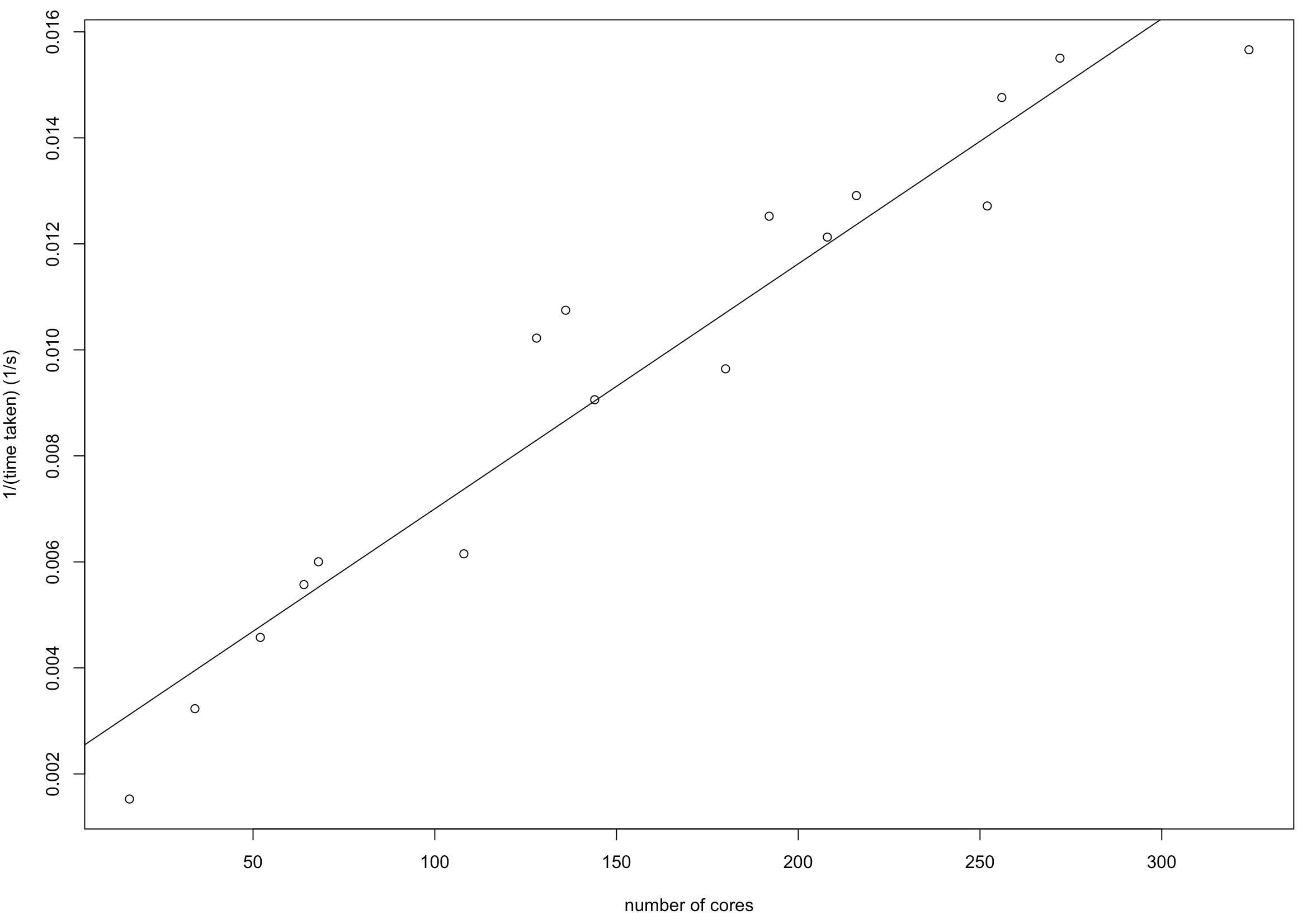
The intercept here is 0.00238 and the slope 0.00004622
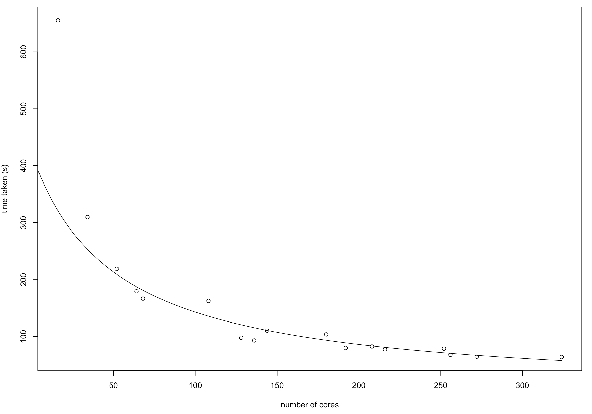
In general for large n, small p data, the run time decreases inversely linearly as the number of cores per executor increases, provided the maximum number of cores isn’t capped. However, for large p, small n, decreasing cores per executor seems to decrease runtime instead. We suspect this could be due to the way data is parallelised in Spark. Currently the method for generating a ‘large p small n’ dataset generate a dataset with a lot of partitions each with a smaller amount of data, as it appends rows iteratively, each of which is an rdd. So it may be more efficient for Mesos to distribute data to more executors but each with a smaller amount of data. This is an area which requires further investigating.
| n | p | cores per executor | Runtime(s) |
|---|---|---|---|
| 100 | 10^5 | 4 | 1107.30 |
| 100 | 10^6 | 4 | 4507.09 |
| 100 | 10^5 | 36 | 2534.42 |
| 100 | 10^6 | 36 | 5176.72 |
Logistic regression
Runtime vs data size
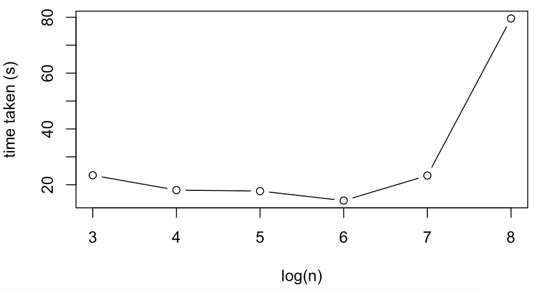
Trends for Logistic regression were mostly similar. For example, run time only increases significantly for large datasizes, albeit the run times are smaller for larger values of n and noiser/larger for small values of n (in the sense that the time for 10^3 was larger than 10^4 despite averaging over several runs).
| n | p | Runtime(s) |
|---|---|---|
| 10^3 | 100 | 23.40 |
| 10^4 | 100 | 18.08 |
| 10^5 | 100 | 17.74 |
| 10^6 | 100 | 14.33 |
| 10^7 | 100 | 23.29 |
| 10^8 | 100 | 79.58 |